Tag Archives: hard drive

Drive Appearance

One of the more common, yet more tricky fundamental concepts in computing today is the concept of drive appearance or, in other words, something that appears to be a hard drive.  This may sound simple, and mostly it is, but it can be tricky.

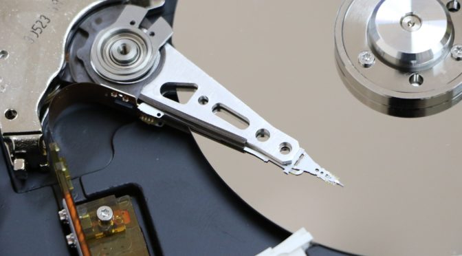
First, what is a hard drive.  This should be simple.  We normally mean a traditional spinning disk Winchester device such have been made for decades in standard three and a half inch as well as two and a half inch form factors.  They contain platters that spin, a drive head that moves forward and backward and they connect using something like ATA or SCSI connectors.  Most of us can pick up a hard drive with our hands and be certain that we have a hard drive.  This is what we call the physical manifestation of the drive.

To the computer, though, it does not see the casing of the drive nor the connectors.  The computer has to look through its electronics and “see” the drive digitally.  This is very, very different from how humans view the physical drive.  To the computer, a hard drive appears as an ATA, SCSI or Fibre Channel device at the most basic physical level and are generally abstracted at a higher level as a block device.  This is what we would call a logical appearance, rather than a physical one.  For our purposes here, we will think of all of these drive interfaces as being block devices.  They do differ, but only slightly and not consequentially to the discussion.  What is important is that there is a standard interface or set of closely related interfaces that are seen by the computer as being a hard drive.

Another way to think of the logical drive appearance here is that anything that looks like a hard drive to the computer is something on which the computer format with a filesystem.  Filesystems are not drives themselves, but require a drive on which to be placed.

The concept of the interface is the most important one here.  To the computer, it is “anything that implements a hard drive interface” that is truly seen as being a hard drive.  This is both a simple as well as a powerful concept.

It is because of the use of a standard interface that we were able to take flash memory, attach it to a disk controller that would present it over a standard protocol (both SATA and SAS implementations of ATA and SCSI are common for this today) and create SSDs that look and act exactly like traditional Winchester drives to the computer yet have nothing physically in common with them.  They may or may not come in a familiar physical form factor, but they definitely lack platters and a drive head.  Looking at the workings of a traditional hard drive and a modern SSD we would not guess that they share a purpose.

This concept applies to many devices.  Obviously SD cards and USB memory sticks work in the same way.  But importantly, this is how partitions on top of hard drives work.  The partitioning system uses the concept of drive impression interface on one side to be able to be applied to a device, and on the other side it presents a drive impression interface to whatever wants to use it; normally a filesystem.  This idea of something that using the drive impression interface on both sides is very important.  By doing this, we get a uniform and universal building block system for making complex storage systems!

We see this concept of “drive in; drive out” in many cases.  Probably the best know is RAID.  A RAID system takes an array of hard drives, applies one of a number of algorithms to make the drives act as a team, and then present them as a single drive impression to the next system up the “stack.”  This encapsulation is what gives RAID its power: systems further up the stack looking at a RAID array see literally a hard drive.  They do not see the array of drives, they do not know what is below the RAID.  They just see the resulting drive(s) that the RAID system present.

Because a RAID system takes an arbitrary number of drives and presents them as a standard drive we have the theoretical ability to layer RAID as many times as we want.  Of course this would be extremely impractical to do to any great degree.  But it is through this concept that nested RAID arrays are possible.   For example, if we had many physical hard drives split into pairs and each pair in a RAID 1 array.  Each of those resulting arrays gets presented as a single drive.  Each of those resulting logical drives can be combined into another RAID array, such as RAID 0.  Doing this is how RAID 10 is built.  Going further we could take a number of RAID 10 arrays, present them all to another RAID system that puts them in RAID 0 again and get RAID 100 and so forth indefinitely.

Similarly the logical volume layer uses the same kind of encapsulation as RAID to work its magic.  Logical Volume Managers, such as LVM on Linux and Dynamic Disks on Windows, sit on top of logical disks and provide a layer where you can do powerful management such as flexibly expanding devices or enabling snapshots, and then present logical disks (aka drive impression interface) to the next layer of the stack.

Because of the uniform nature of drive impressions the stack can happen in any order.  A logical volume manager can sit on top of RAID, or RAID can sit on top of a logical volume manager and of course you can skip or the other or both!

The concept of drive impressions or logical hard drives is powerful in its simplicity and allows us great potential for customizing storage systems however we need to make them.

Of course there are other uses of the logical drive concept as well.  One of the most popular and least understood is that of a SAN.  A SAN is nothing more than a device that takes one or more physical disks and presents them as logical drives (this presentation of a logical drive from a SAN is called a LUN) over the network.  This is, quite literally, all that a SAN is.  Most SANs will incorporate a RAID layer and likely a logical volume manager layer before presenting the final LUNs, or disk impressions, to the network, but that is not required to be a SAN.

This means, of course, that multiple SAN LUNs can be combined in a single RAID or controlled via a logical volume layer.  And of course it means that a SAN LUN, a physical hard drive, a RAID array, a logical volume, a partition…. can all be formatted with a filesystem as they are all different means of achieving the same result.  They all behave identically.  They all share the drive appearance interface.

To give a real world example of how you would often see all of these parts come together we will examine one of the most common “storage stacks” that you will find in the enterprise space.  Of course there are many ways to build a storage stack so do not be surprised if yours is different.  At the bottom of the stack is nearly always physical hard drives, which could include solid state drives.  This are located physically within a SAN.  Before leaving the SAN the stack will likely include the actual storage layer of the drives, then a RAID layer combining those drives into a single entity.  Then a logical volume layer to allow for features like growth and snapshots.  Then there is the physical demarcation between the SAN and the server which is presented as the LUN.  The LUN then has a logical volume manager applies to it on the server / operating system side of the demarcation point.  Then on top of that LUN is a filesystem which is our final step as the filesystem does not continue to present a drive appearance interface but a file interface, instead.

Understanding drive appearance, or logical drives, and how these allows components to interface with each other to build complex storage subsystems is a critical building block to IT understanding and is widely applicable to a large number of IT activities.

Practical RAID Choices for Spindle Based Arrays

A truly monumental amount of information abounds in reference to RAID storage systems exploring topics such as risk, performance, capacity, trends, approaches and more.  While the work on this subject is nearly staggering the information can be distilled into a handful of common, practical storage approaches that will cover nearly all use cases.  My goal here is to provide a handy guide that will allow a non-storage practitioner to approach RAID decision making in a practical and, most importantly, safe way.

For the purposes of this guide we will assume storage projects of no more than twenty five traditional drives (spinning platter drives properly known as Winchester drives.)  These drives could be SFF (2.5″) or LFF (3.5″) commonly, SATA or SAS, consumer or enterprise.  We will not tackle solid state drives as these have very different characteristics and require their own guidance.  Storage systems larger than roughly twenty five spindles should not work from standard guidance but delve deeper into specific storage needs to ensure proper planning.

The guidance here is written for standard systems in 2015.  Over the past two decades the common approaches to RAID storage have changed dramatically and while it is not anticipated that the key factors that influence these decisions will change enough in the future to alter these recommendations it is very possible that they will.  Good RAID design of 1998 is very poor RAID design today.  The rate of change in the industry has dropped significantly since that time and these recommendations are likely to stand for a very long time, very possibly until spindle-based drive storage is no longer available or at least popular, but like all things predictions are subject to great change.

In general we use what is termed a “One Big Array” approach.  That is a single RAID array on which all system and data partitions are created.  The need or desire to split our storage into multiple, physical arrays is mostly gone today and should only be done in non-general circumstances.  Only in situations where careful study of the storage needs and heavy analysis are being done should we look at array splitting.  Array splitting is far more likely to cause harm rather than good.  When it doubt, avoid split arrays.  The goal of this guide is general rules of thumb to allow any IT Pro to build a safe and reliable storage system.  Rules of thumb do not and can not cover every scenario, exceptions always exist.  But the idea here is to cover the vast majority of cases with tried and true approaches that are designed around modern equipment, use cases and needs while being mindful to err on the side of safety – when a choice is less than ideal it is still safe.  None of these choices is at all reckless, at worst they are overly conservative.

The first scenario we should consider is if your data does not matter.  This may sound like an odd thing to consider but it is a very important scenario.  There are many times where data saved to disk is considered ephemeral and does not need to be protected.  This is common for reconstructable data such as working space for rendering, intermediary calculation spaces or caches – situations where spending money to protect data is wasted and it would be acceptable to simply recreate lost data rather than protecting it.  This could be a case where downtime is not a problem and data is static or nearly so and rather than spending to reduce downtime we only worry about protecting the data via backup mechanisms so that if an array fails we simply restore the array completely.  In these cases the obvious choice is RAID 0.  It is very fast, very simple and provides the most cost effective capacity.  The only downside of RAID 0 is that it is fragile and provides no protection against data loss in case of drive failure or even a URE (which would cause data corruption the same as a desktop drive faces.)

It should be noted that an exception to the “One Big Array” approach that would be common is in systems using RAID 0 for data.  There would be a very good argument made for a small drive array dedicated to the OS and application data that would be cumbersome to reinstall in case of array loss being kept on RAID 1 and the RAID 0 data array being separate from it.  This way recovery could be very rapid rather than needing to completely rebuild the entire system from scratch rather than simply recreating the data.

Assuming that we have eliminated cases where the data does not require protection, we will assume for all remaining cases that the data is quite important and we want to protect it at some cost.  We will assume that protecting the data as it exists on the live storage is important, generally because we want to avoid downtime or because we want to ensure data integrity because the data on disk is not static and an array failure would also constitute data loss.  With this assumption we will continue.

If we have an array of only two disks the answer is very simple, we choose RAID 1.  There is no other option at this size, so no decision to be made.   In theory we should be planning our arrays holistically and not after the number of drives is determined, the number of drives and the type of array chosen should be done together not drives purchased then use determined based on that arbitrary number, but two drive chassis are so common that it is worth mentioning as a case.

Likewise, with a four drive array the only real choice to consider is RAID 10.  There is no need for further evaluation.  Simply select RAID 10 and continue.

An awkward case is a three drive array.  It is very, very rare that we are limited to three drives as the only common chassis limited to three drives was the Apple Xserve and this has been off of the market for some time so the need to deal with decision making around three spindle arrays should be extremely unlikely.  In cases where we have three drives it is often best to seek guidance but the most common approaches are to add a fourth drive and ergo chose RAID 10 or, if capacity of greater than a single drive’s worth is not needed, to put all three drives into a single triple-mirror RAID 1.

For all other cases, therefore, we are dealing with five to twenty five drives.  Since we have eliminated the situations where RAID 0 and RAID 1 would apply we are left with all common scenarios coming down to RAID 6 and RAID 10, and these constitute the vast majority of cases.  Choosing between RAID 6 and RAID 10 becomes the biggest challenge that we will face as we must look solely at a our “soft” needs of reliability, performance and capacity.

Choosing between RAID 6 and RAID 10 should not be incredibly difficult.  RAID 10 is ideal for situations where performance and safety are the priorities.  RAID 10 has much faster write performance and is safe regardless of disk type used (low cost consumer disks can still be extremely safe, even in large arrays.)  RAID 10 scales well to extremely large sizes, much larger than should be implemented using rules of thumb!  RAID 10 is the safest of all choices, it is fast and safe.  The obvious downsides are that RAID 10 has less storage capacity from the same disks and is more costly on the basis of capacity. It must be mentioned that RAID 10 can only utilize an even number of disks, disks are added in pairs.

RAID 6 is generally safe and fast but never as safe or as fast as RAID 10.  RAID 6 specifically suffers from write performance so is very poorly suited for workloads such as databases and heavily mixed loads like in large virtualization systems.  RAID 6 is cost effective and provides a heavy focus on available capacity compared to RAID 10.  When budgets are tight or capacity needs dominate over performance RAID 6 is an ideal choice.  Rarely is the difference in safety between RAID 10 and RAID 6 a concern except in very large systems with consumer class drives.  RAID 6 is subject to additional risk with consumer class drives that RAID 10 is not affected by which could warrant some concern around reliability in larger RAID 6 systems such as those above roughly 40TB when consumer drives are used.

In the small business space especially, the majority of systems will use RAID 10 simply because arrays rarely need to be larger than four drives.  When arrays are larger RAID 6 is the more common choice due to somewhat tight budgets and generally low concern around performance.  Both RAID 6 and RAID 10 are safe and effective solutions for nearly all usage scenarios with RAID 10 dominating when performance or extreme reliability are key and RAID 6 dominating when cost and capacity are key.  And, of course, when storage needs are highly unique or very large, such as larger than twenty five spindles in an array, remember to leverage a storage consultant as the scenario can easily become very complex.  Storage is one place where it pays to be extra diligent as so many things depend upon it, mistakes are so easy to make and the flexibility to change it after the fact is so low.

Understanding the Western Digital SATA Drive Lineup (2014)

I choose to categorize Western Digital’s SATA drive lineup for several reasons. One is that WD is the current market leader in spinning hard drives so this makes the categorization most useful to the greatest number of people, the “color coded” line is, based on anecdotal evidence, far and away the chosen drive family of the small business market where the diagnosis is most important and SATA drives retain the most disparity of features and factors making them far more necessary to understand well. While technically the only difference between a SAS (SCSI) and SATA (ATA) drive or even a Fibre Channel (FC) drive is nothing but the communications protocol used to communicate with them, in practical terms SAS and FC drives are only made in certain, high reliability configurations and do not require the same degree of scrutiny and do not carry the same extreme risks as SATA drives. Understanding SATA drive offerings is the more important for practical, real world storage needs.

WD has made understanding their SATA drive line up especially easy by adding color codes to the majority of their SATA drive offerings – those deemed to be “consumer” drives, and an “E” designation on their enterprise SATA drives and one outlier, the high performance Velociraptor drives which seek to compete with common SAS performance for SATA controllers. Altogether they have seven SATA drive families to consider covering the gamut of drive factors. While this diagnosis will apply to the easy to understand WD lineup, by comparing factors here with the offerings of other drive makers the use cases of their drives can be determined as well.

In considering SATA drives, three really key factors stand out as being the most crucial to consider (outside of price, of course.)

URE Rate: URE, or Unrecoverable Read Error, is an event that happens, with some regularity, to electromechanical disk storage media where a single sector is unable to be retrieved. In a standalone drive this happens from time to time but generally only affects a single file and users typically see this as a lost file (often one they do not notice) or possible a corrupt filesystem which may or may not easily be corrected. In healthy RAID arrays (other than RAID 0), the RAID system provides mirroring and/or parity that can cover for this sector failure and recreate the data protecting us from URE issues. When a RAID array is in a degraded state UREs are a potential risk again. In its worst case, a URE on a degraded parity array can, in some cases, cause total loss of an array (all data is lost.) So considering UREs and their implications in any drive purchases is extremely important and is the primary driver of cost differential in drives of varying types. URE varies from the low end at 10^14 to the high end at 10^16. The numbers are so large that they are always written in scientific notation. I will not go into an in-depth explanation of URE rates, ramifications and mitigation strategies here, but understanding URE is critical to decision making around drive purchases, especially in the large capacity, lower reliability space of SATA drives.

Spindle Speed: This is one of the biggest factors to most users, spindle speed directly correlates to IOPS and throughput. While measurements of drive speed are dynamic, at best, spindle speed is the best overall way to compare two otherwise identical drives under identical load. A 15,000 RPM drive will deliver almost exactly double the IOPS and throughput of a 7,200 RPM drive, for example. SATA drives commonly come in 5,400 RPM and 7,200 RPM varieties with rare high performance drives available at 10,000 RPMs.

Error Recovery Control (ERC): Also known as TLER (Time Limited Error Recovery) in WD parlance, ERC is a feature of a drive’s firmware which allows for configurable time limits for read or write errors which can be important when a hard drive is used in a RAID array as often error recovery needs to be handled at the array, rather than the drive, level. Without ERC, a drive is more likely to be incorrectly marked as failed when it has not. This is most dangerous in hardware based parity RAID arrays and has differing levels of effectiveness based on individual RAID controller parameters. It is an important feature for drives assumed for use in RAID arrays.

In addition to these key factors, WD lists many others for their drives such as cache size, number of processors, mean time between failures, etc. These tend to be far less important, especially MTBF and other reliability numbers as these can be skewed or misinterpreted easily and rarely offer the insight into drive reliability that we expect or hope. Cache size is not very significant for RAID arrays as they need to be disabled for reasons of data integrity. So outside of desktop use scenarios, the size of a hard drive’s cache is generally considered irrelevant. CPU count could also be misleading as single CPUs may be more powerful than dual CPUs if the CPUs are not identical and the efficacy of the second CPU is unknown. But WD lists this as a prominent feature of some drives and it is assumed that there is measurable performance gain, most likely in latency reduction, through the addition of the second CPU. I do, however, continue to treat this as a trivial factor and mostly only useful as a point of interest rather than as a decision factor
The drives.

All color-coded drives (Blue, Green, Red and Black) share one common factor – they have the “consumer” URE rating of 10^14. Consumer is a poor description here but is, more or less, industry standard. A better description is “desktop class” or suitable for non-parity RAID uses. The only truly poor application of 10^14 URE drives is in parity RAID arrays and even there, they can have their place if properly understood.

Blue: WD Blue drives are the effective baseline model for the SATA lineup. They spin at the “default” 7,200 RPMs, lack ERC/TLER and have a single processor. Drive cache varies between 16MB, 32MB and 64MB depending on the specific model. Blue drives are targeted at traditional desktop usage – as single drives with moderate speed characteristics, not well suited to server or RAID usage. Blue drives are what is “expected” to be found in off the shelf desktops. Blue drives have widely lost popularity and are often not available in larger sizes. Black and Green drives have mostly replaced the use of Blue drives, at least in larger capacity scenarios.

Black: WD Black drives are a small upgrade to the Blue drives changing nothing except to upgrade from one to two processors to slightly improve performance while not being quite as cost effective. Like the Blue drives they lack ERC/TLER and spin at 7,200 RPM. All Black drives have the 64MB cache. As with the Blue drives, Black drives are most suitable for traditional desktop applications where drives are stand alone.

Green: WD Green drives, as their name nominally implies, are designed for low power consumption applications. They are most similar to Blue drives but spin at a slower 5,400 RPMs which requires less power and generates less heat. Green drives, like Blue and Black, are designed for standalone use primarily in desktops that need less drive performance than is expected in an average desktop. Green drives have proven to be very popular due to their low cost of acquisition and operation. It is assumed, as well, that Green drives are more reliable than their faster spinning counterparts due to the lower wear and tear of the slower spindles although I am not aware of any study to this effect.

Red: WD Red drives are unique in the “color coded” WD drive line up in that they offer ERC/TLER and are designed for use in small “home use” server RAID arrays and storage devices (such as NAS and SAN.) Under the hood the WD Red drives are WD Green drives, all specifications are the same including the 5,400 RPM spindle speed, but with TLER enabled in the firmware. Physically they are the same drives. WD officially recommends Red drives only for consumer applications but Red drives, due to their lower power consumption and TLER, have proven to be extremely popular in large RAID arrays, especially when used for archiving. Red drives, having URE 10^14, are dangerous to use in parity RAID arrays but are excellent for mirrored RAID arrays and truly shine at archival and similar storage needs where large capacity and low operational costs are key and storage performance is not very important.

Outside of the color coded drives, WD has three SATA drive families which are all considered enterprise. What these drives share in common is that their URE rate is much higher than that of the “consumer” color coded drives. Ranging from URE 10^15 to 10^16 depending on model. The most important result of this URE rate is that these drives are far more applicable to use in parity RAID arrays (e.g. RAID 6.)

SE: SE drives are WD’s entry level enterprise SATA drives with URE 10^15 rates and 7,200 RPM spindle speeds. They have dual processors and a 64MB cache. Most importantly, SE drives have ERC/TLER enabled. SE drives are ideal for enterprise RAID arrays both mirrored and parity.

RE: RE drives are WD’s high end standard enterprise SATA drives with all specifications being identical to the SE drives but with the even better URE 10^16 rate. RE drives are the star players in WD’s RAID drive strategy being perfect for extremely large capacity arrays even when used in parity arrays. RE drives are available in both SATA and SAS configurations but with the same drive mechanics.

Velociraptor: WD’s Velociraptor is a bit of an odd member of the SATA category. With URE 10^16 and a 10,000 RPM spindle speed the Velociraptor is both highly reliable and very fast for a SATA drive competing with common, mainline SAS drives. Surprisingly, the Velociraptor has only a single processor and even more surprisingly, it lacks ERC/TLER making it questionable for use in RAID arrays. Lacking ERC, use in RAID can be considered on an implementation by implementation basis depending on how the RAID system interacts with the drive’s timing. With the excellent URE rating, Velociraptor would be an excellent choice for large, higher performance parity RAID arrays but only if the array handles the error timing in a graceful way, otherwise the risk of the array marking the drive as having failed is unacceptably high for an array as costly as this would be. It should be noted that Velociraptor drives do not come in capacities comparable to the other SATA drive offerings – they are much smaller.

Of course the final comparison that one needs to make is in price. When considering drive purchases, especially where large RAID arrays are concerned or for other bulk storage needs, the per drive cost is often a major, if not the driving, factor. The use of slower, less reliable drives in a more reliable RAID level (such as Red drives in RAID 10) versus faster, more reliable drives in a less reliable RAID level (such as RE drives in RAID 6) often provides a better blend of reliability, performance, capacity and cost. Real world drive prices play a significant factor in these decisions. These prices, unlike the drive specifications, can fluctuate from day to day and swing planning decisions in different directions but, overall, tend to remain relatively stable in comparison to one another.

At the time of this article, at the end of 2013, a quick survey of prices of 3TB drives from WD give these approximate breakdown:

Green $120
Red $135
Black $155
SE $204
RE $265

As can be seen, the jump in price primarily comes between the consumer or desktop class drives and the enterprise drives with their better URE rates with Red and RE drives, both with ERC/TLER, being in a price ratio of almost exactly 2:1 making, for equal capacity, it favorable to choose many more Red drives in RAID 10 than fewer RE drives in RAID 6, as an example. So comparing a number of factors, along with current real world prices, is crucial to making many buying decisions.

Newer drives, just being released, are starting to see reductions in onboard drive cache for exactly the reasons we stated above, drives designed around RAID use have little or no purpose to having onboard cache as it needs to be disabled for data integrity purposes.

Drive makers today are offering a wide variety of traditional spindle-based drive options to fit many different needs. Understanding these can lead to better reliability and more cost effective purchasing and will extend the usefulness of traditional drive technologies into the coming years.